{sf} - Plotting Spatial Objects

Almost every time I try to stack geometries when plotting {sf} objects I try to use the syntax below. This doesn't seem to work, and doesn't throw any errors. I don't understand why.

library(sf)

nz <- spData::nz
nz_height <- spData::nz_height

plot(nz[0])
plot(nz_height[0], add = T)

I've found the only way to plot geometries on the same plot is to use st_geometry within the plot function. st_geometry function extracts the geometry from the sf object. In the code below I've styled the map to better distinguish the points from the polygons.

plot(st_geometry(nz[nz$Island == 'South', ]), col = '#9a00fa', border = '#c871ff')
plot(st_geometry(nz_height), col = 'mediumspringgreen', cex = 1.5, add = T)

What about coloring elements in the geometry based an attribute? Let's use some new data too. I've used the {tigris} package to download some US Census data.

library(sf)
us_states <- tigris::states(class = 'sf')
us_west <- us_states[us_states$NAME %in% c('Washington', 'Oregon', 'California'), ]

roads <- tigris::primary_roads(class = 'sf')
roads <- roads[us_west, ]

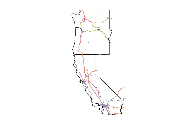
plot(st_geometry(us_west))
plot(roads['RTTYP'], add = T)

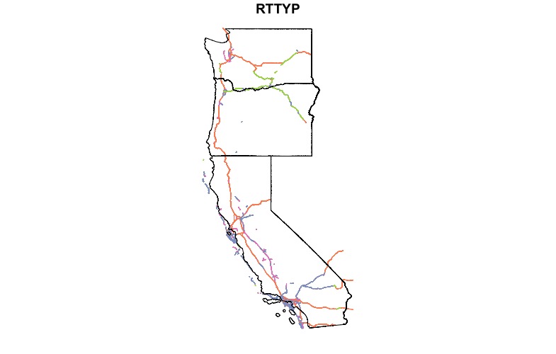
Although, you'll need to check the order of the you plot the geometries. I can't figure out why this happens. Maybe it is just an issue with my install of R or {sf}.

plot(roads['RTTYP'])
plot(st_geometry(us_west), add = T)

I need to experiment more with base R plotting to figure this out.

{ggplot2}

I generally plot using {ggplot2}, and the best thing about {sf} is that it includes methods to plot spatial objects with {ggplot2}. As much as I plot with {ggplot2}, I haven't used it very frequently with {sf} objects. If you are used to plotting in {ggplot} it shouldn't be too different than what you're used to.

library(ggplot2)

ggplot() +
  geom_sf(data = us_west, fill = NA) +
  geom_sf(data = roads, aes(color = RTTYP)) +
  coord_sf() +
  theme_void()

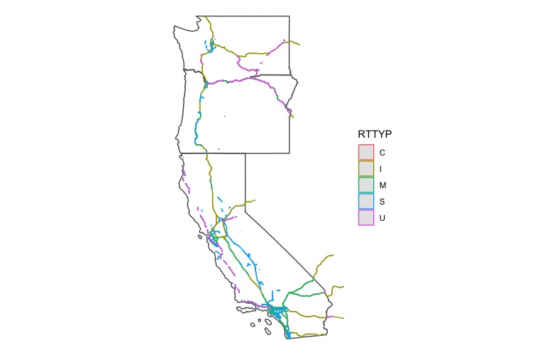
Pretty much any of the methods you would use with {ggplot2}.

Easy Interactive Maps

One last tip for this post. The {mapview} library has a great general purpose mapping function, mapview. It will plot {sf} objects as an interactive Leaflet map. If you provide the name of a column in the function call, mapview(us_states['NAME']) it'll color the states just like base R plotting of {sf} objects. As an added bonus, the mapview function will add popups and tooltips to the map. Super handy! I genuinely love this function because it helps me avoid using ArcMap or QGIS to quickly visualize shapefiles.

library(mapview)

# doesn't color states, includes all attributes in popup
mapview(us_west)

# colors states based on provided attribute,
# doesn't include all attributes in popup
mapview(us_west['NAME'])

Alternatives

There are a few plotting alternatives, but those mentioned above are the simplest. {tmap}, or thematic maps, provides a {ggplot2} like interface for plotting. The {leaflet} library is a wrapper for the Leaflet javascript library. It is more complicated than using the {mapview} library, but it is more customizable.

There you have it, a few different methods of plotting spatial data in R. While not a comprehensive tutorial on visualizing spatial data, it should be enough to get started. And it will help me remember to use st_geometry when plotting {sf} objects.